Pipeline · the centerpiece
From caw to cluster.
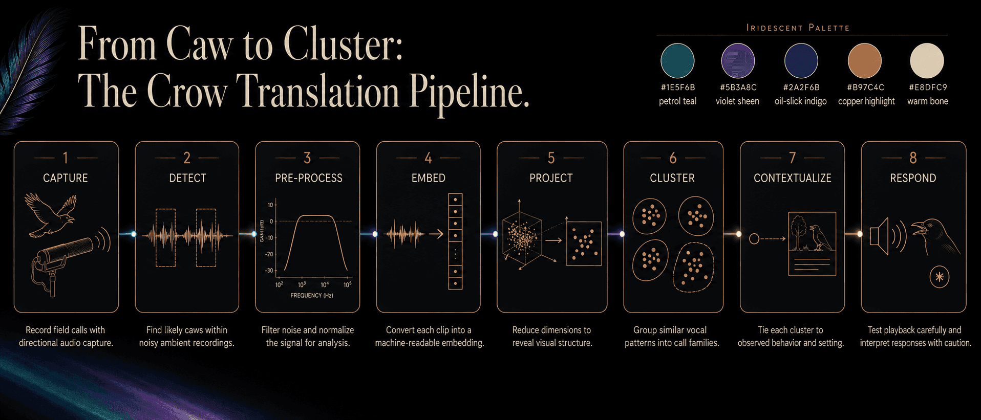
How a 30-second phone recording becomes an interpretable map of a crow's vocal repertoire — in eight stages, with the failure modes named alongside each step.
Capture — record the call without breaking the scene.
Audio quality is the floor of every downstream model. Field-recording discipline pays compound interest.
You only get one chance at the take. Sample rate, mic placement, behavioral context, and exact timestamp matter more than any post-processing step. Sync the recorder clock to the phone running your behavior log; you'll join them at stage 6.
▸ Show code — bashbash
# Field rig — 48 kHz / 24-bit, mono, lossless
ffmpeg -f avfoundation -i ":1" -ar 48000 -ac 1 -c:a pcm_s24le \
  -metadata location="Discovery Park, Seattle (city-coarsened)" \
  -metadata recordist="J. Field" \
capture_$(date +%s).wavDetect — find every vocalization in the file.
Long recordings are mostly silence and ambient noise. Detection narrows hours of audio down to seconds of crow.
BirdNET-Analyzer, Perch, and NatureLM-audio all do this. BirdNET is the workhorse: fast, mature, multi-species. Perch and NatureLM-audio have better recall on graded calls but cost more compute. Pick by your audio volume.
▸ Show code — pythonpython
from birdnet_analyzer import analyze

hits = analyze(
    path="capture_001.wav",
    species_list=["Corvus brachyrhynchos"],
    min_confidence=0.4,
)
# → list of (start_s, end_s, confidence)Preprocess — clean what you got, conservatively.
Heavy denoising distorts the signal an SSL model wants to read. Light, reversible, transparent is the rule.
A bandpass from 200 Hz to 8 kHz brackets crow energy without cutting harmonics. Peak-normalize, don't loudness-normalize — context-relative loudness encodes urgency.
▸ Show code — pythonpython
import librosa, noisereduce as nr

y, sr = librosa.load("clip.wav", sr=48000, mono=True)
y = librosa.effects.preemphasis(y)
y = nr.reduce_noise(y=y, sr=sr, stationary=False, prop_decrease=0.6)
y = librosa.util.normalize(y)Embed — a clip becomes 1,024 numbers in a learned space.
A 30-second clip becomes a 1,024-number list. That sounds like a downgrade. It isn't.
The 1,024 numbers are coordinates in a space the model built itself, by listening to millions of audio clips and learning what makes any clip distinct from any other. Crow caws that sound alikeend up close together. Caws that differ in context end up apart. We don't tell the model what to look for. It tells us.
▸ Show code — pythonpython
from naturelm_audio import NatureLM

model = NatureLM.from_pretrained("EarthSpeciesProject/NatureLM-audio")
emb = model.embed("./crow_clip_001.wav")
# emb : np.ndarray, shape (1024,)Project — collapse 1,024 dimensions to two you can see.
UMAP and friends compress high-dimensional structure into a 2-D map a human can read. Some of the geometry survives. Some doesn't.
Projection is a lossy summary of geometry, not a ground truth. Use it for inspection and overview; do downstream math (similarity, clustering) on the original embeddings.
▸ Show code — pythonpython
import umap

proj = umap.UMAP(
    n_neighbors=15,
    min_dist=0.0,
    metric="cosine",
    random_state=42,
).fit_transform(embeddings) # shape (n, 2)Cluster — let the densities tell you the categories.
HDBSCAN finds dense regions without forcing a target count. Call types emerge as clusters; graded calls show up as bridges between them.
Run clustering on the full 1,024-dim embeddings, not the 2-D projection. Display on the projection. The cluster IDs become your working repertoire — refine with a human ear at the next stage.
▸ Show code — pythonpython
import hdbscan

labels = hdbscan.HDBSCAN(
    min_cluster_size=20,
    metric="euclidean",
    cluster_selection_method="leaf",
).fit_predict(embeddings) # noise → -1Contextualize — join clusters to behavior.
A cluster is just a number until you join it to the video, the GPS, or the behavior log. Context is what turns geometry into meaning.
The Demartsev et al. (2026) carrion-crow paper is the cleanest recent example: wearable loggers gave them per-individual synchronized behavior + audio, so cluster ↔ context maps were recoverable at scale.
cluster 07 · Loud grunt
Foraging 62% · Affiliative 21% · Other 17%
cluster 02 · Caw — long
Territorial 74% · Alarm 11% · Other 15%
cluster 11 · Rattle
Affiliative 49% · Recruitment 31% · Other 20%
▸ Show code — pythonpython
# join cluster labels to behavior log via timestamp window
calls["cluster"] = labels
contexts = calls.merge(behavior, on="time_window", how="left")
ctx_probs = (
    contexts.groupby("cluster")["behavior"]
            .value_counts(normalize=True)
)Respond — playback as a calibrated experiment, not an Instagram trick.
A playback session is data collection. Treat it like one: pre-registered, observed, time-bounded, halted on distress.
Bidirectional dialogue is on the roadmap. For v0 we ship a tightly-bounded one-way protocol: play a known exemplar, video the reaction, log the timestamps, publish raw and methods both.
▸ Show code — pythonpython
from crowlingo.playback import PlaybackSession

session = PlaybackSession(
    stimulus="cluster_07_exemplar.wav",  # "loud grunts"
    max_seconds=60,
    distance_m=20,
    observer=video_observer,
    distress_callback=halt,
)
session.run()The pipeline, end-to-end
Eight stages, one map, an ear at every step.
The atlas is the artifact. Each crow vocalization in your recordings becomes a point in the same shared space — visible, comparable, queryable, listenable.